Motion 🚗

A Descriptive Model for Particles

AP Physics 2026-27 with Mr. Porter

Contents

Buggy Lab 🚗

Objective:

  • Determine if your toy buggy moves in a consistent manner by developing a relationship between position and time.
  • Use time as your independent variable

Lab Results:

  • The buggies moved with a constant velocity
    • means that it changed its position equal amounts for each equal change in time
  • Velocity () is represented by the slope of the position vs. time graph
    • how "fast"
    • AND what direction
  • Speed is the steepness of the slope:
    • it tells us the rate that position changes with time
    • steeper slope == faster
  • The initial position ( or ) of the object is the vertical intercept
    • it tells us where the object is at clock reading 0.

Mathematical Models

General Mathematical Mode:

Specific Mathematical Model (example):

Narrative Model:

"The toy car started at a position of 250 cm and moved in the positive direction at a speed of 25 cm/s."

Vector vs. Scalar

Vector

  • Physical Quantity that describes magnitude (size) and direction
  • indicated with an ➡️ above the symbol
    • i.e. or or

Scalar

  • Physical quantity that describes the magnitude (size) of something

Defining "How Far"

Who went further? Dorothy or Toto?

center

Position

  • Where an object is at any particular time in coordinate system (vector)
  • "Location"

Displacement

  • Change in position of an object
  • Includes direction (vector quantity)

Distance

  • the magnitude (or size) of displacement between two positions (scalar quantity)
  • more often referred to as distance traveled which is the total length of the path traveled between two positions

Demo - vs.

Speed vs. Velocity:

  • Velocity is a vector quantity
    • how fast and what direction
  • Speed is a scalar quantity
    • how fast

Analyzing Position-Time (XT) Graphs

For the following position vs. time graph, consider the positive direction to be north.

  1. When is the object moving North? South?
  2. When is the object stopped?
  3. When is the object North of the origin?
  4. What is the velocity of the object at s? s? s? When it is at the origin?
  5. When does the object change directions?

Average vs. Instantaneous

  • Average - what is something over a period of time,
  • Instantaneous - what is something at that exact moment in time,

Velocity vs. Speed

Average Velocity

Average Speed

Instantaneous Values:

  • "at that moment"
  • Value at a specific time

Instantaneous Velocity

  • Velocity at a specific time
  • The slope of the position vs. time graph at that time measurement

Instantaneous Speed

  • Magnitude of the velocity

Visualizing Instantaneous Velocity

center

Average vs. Instantaneous Demo Page

Analyzing Position-Time (XT) Graphs

  1. What is the total distance the object travels?
  2. What is the total displacement of the object?
  3. What is the average velocity of the object?
  4. What is the average speed of the object?

Average Velocity

Dispalcement divided by the change in time.

"The average slope of the graph"

Average Speed

Total distance divided by change in time

Mathematical Models

  • - position
  • - average velocity
  • - instantaneous time
  • - initial position, position at .

Problem Solving with Mathematical Models:

A red car (top) and a green car (bottom) are having a race. The green car has a head start (distance a). The two cars start at the same time. The red car must travel to the finish line (distance b). The red car averages a speed of . The green car averages a speed of .

  1. Determine the time it takes the red car to reach the finish line.
  2. Determine the time it takes the green car to reach the finish line.

center

Velocity vs. Time Graphs

How Far Did It Go?

Reading displacement off a velocity graph

You Already Know This One

A cart rolls at a steady 6 m/s. How far does it go in the first 4 seconds?

center

Ground Rules for the Next Hour

  • There is no new formula on this handout. You already have what you need
  • Write down answers you are not sure about. You can fix them later
  • Argue with your group. Out loud
  • When you ask me "is this right?", I am going to ask you how you'd check

Your job today is not to remember a rule. It is to build one.

One Slice at a Time

center

Inside a single slice the cart is never at one steady speed. To use
you have to pick one speed to stand in for the whole
slice — and there are three sensible picks.

Same Rule, Every Slice

center

Pick your rule, then apply it to every slice without changing your mind
part-way along.

How to Draw One

  1. Mark the slice edges on the time axis
  2. Take one slice. Find where the line crosses its left edge and its right edge
  3. Low: draw a horizontal line across the slice at the slower of those two.
    High: at the faster. Midpoint: go up to the line from the middle of the slice
  4. Close the rectangle down to the time axis
  5. Area height width. The width is the same every time — only the height changes

On a line that falls, the slower end is the right-hand one. Ask which end is
slower, never which end is on the left.

Nobody Told You the Rule

You built it yourselves.

Here is what you found, in the order you found it.

Three Rectangles, One Total

Constant velocity in each piece, so works on each piece.

Interval 0 → 2 s 2 → 5 s 5 → 8 s
Velocity 8 m/s 2 m/s 5 m/s
Displacement 16 m 6 m 15 m

Total: 37 m — and each piece is a rectangle you could have measured.

Area Here Is Rise There

center

The 16 m you found as an area on the right is the 16 m the cart climbs
on the left. One displacement, drawn two ways.

Backwards Counts Too

center

Still rectangles, still constant velocity — but one of them sits below the
axis
. A geometric area is never negative. That displacement is.

Then We Broke It

A cart starts from rest and reaches 12 m/s in 6 seconds.

There isn't one. The velocity is different at every instant.

The formula is not wrong. It needs a that holds still — and this
graph never gives it one.

Why Rectangles?

needs a velocity that holds still. Over the whole 6 seconds nothing does — but over a short enough stretch, it barely moves.

  • Chop the 6 s into slices
  • Inside one slice, pretend the velocity is constant
  • A rectangle is that pretence: one height, held for one slice

Every rectangle is a deliberate lie. The whole method rests on telling one
whose direction you already know.

Three Ways to Guess

center

Low falls short in every slice, so the total must be too small. High overshoots in every slice, so it must be too big. The answer is trapped.
The midpoint is wrong in two directions at once, by equal amounts.

Squeeze It

center

Thinner slices, smaller lie. The floor rises, the ceiling drops, and the trap
closes on the answer from both sides at once.

Why the Gap Halves

Upper and lower sums share every interior rectangle. They differ by exactly
one — height , width :

Slices Gap
2 3 s 36 m
4 1.5 s 18 m
8 0.75 s 9 m

Halve the slice, halve the gap. Keep going and the bracket closes on one number.

What If the Line Bends?

center

Nothing changes. Low is still a floor, high is still a ceiling, and the gap still halves when you halve .

Two Roads, One Number

center

Geometry: m
Average velocity: m/s, so m

Two methods that share no steps, agreeing. That is why you can trust a rule
nobody handed you.

The Rule

The displacement over an interval is the area between the graph and the
time axis — counting area above the axis as positive and below as negative.

All three of those phrases are load-bearing.

Signs Are Not Decoration

center

  • Displacement keeps the signs, and they cancel → 0 m
  • Distance ignores the signs and adds the sizes → 18 m

Same graph. Two different questions. Read which one you were asked.

The Units Were Never Going to Allow Anything Else

Area on this graph has to come out in meters. Meters are what displacement is
measured in.

A rule that produced seconds, or m/s, could not possibly have been giving you
a displacement. The units were telling you before the arithmetic did.

Two Graphs, Two Tools

Look at Gives you
Slope a position–time graph velocity (m ÷ s)
Area a velocity–time graph displacement (m/s × s)
  • How fast is it going? → slope of the position graph
  • How far did it get? → area under the velocity graph

Check the units of what you were asked for. They pick the tool for you.

Harder Graphs, Same Rule

In Part C the lines sloped, so the regions were triangles and trapezoids
instead of rectangles. Some of them sat below the axis.

Nothing else changed. Find the region, find its area, keep the sign.

Same Size, Opposite Direction

center

Two carts, two regions of equal area, on opposite sides of the time axis.
One ends up 64 m ahead, the other 64 m behind. The sign is the direction.

Where This Comes Back

Multiply the two axes together and the area carries their product's unit.

  • velocity time → displacement
  • force position → work, in Unit 3

The move you invented today is not about velocity. It is what area always
means when the two axes multiply to something you care about.

Fan Carts

1. Observations

  1. What do you notice about the motion?

2. Questions

  1. What questions could you ask about the motion?

3. Measurements

  1. What would you measure to answer those questions?

Essential Questions 🤔

  • Does your the fan cart change its velocity?

  • If it does change velocity, does the velocity change constantly?

  • What evidence do you need to collect to answer these questions?

Some New Tools 🧰 🛠️

Spark Timer 🎇

  1. Tape spark tape to object
  2. Pick time setting
  3. Turn on timer & object and send it

Essential Questions 🤔

  • Does your the fan cart change its velocity?

  • If it does change velocity, does the velocity change constantly?

  • What evidence do you need to collect to answer these questions?


Hypothesis

  • Make an hypothesis answering the essential questions, add why you think that and what your graph/data would look like to support your hypothesis

Finding Velocity from Position time Graphs

  • Reminder: the slope at a specific time on a position vs. time graph is the instantaneous velocity of an object

  • Why can't we just use ?

Create a Velocity vs. Time Graph from your Data

From your Velocity vs. Time Graph...

Does your object change its velocity?

If it does change velocity, does the velocity change constantly?

  • What does the slope represent?
  • What does the intercept represent?

Kinematic Graphs

What about Position and Time?

What is the relationship betwen position and time?

How do we know what curve to pick??

Linearization

Linearization is the art of transforming curved relationships into straight lines.

Why Linearize?

  1. Finding constants is easy - The slope of a straight line directly gives you physical constants (like , , or )
  2. Checking your model - A straight line confirms you have the right equation (high R² value = good fit!)
  3. Making predictions - It's much easier to extrapolate from a straight line than a curve

Linearizing allows us to interpret

curves as lines

How do we change a curve into a line?

By making a test plot

  1. Make a new data column
  2. Calculate the expected relationship in that column (i.e. if the graph looks quadratic calculate )
  3. Make a new plot (i.e. graph vs. )
  4. Analyze new linear model

Example & Demo

Cheat Sheet

Class Data Questions:

  1. What does the VT slope represent?
  2. Does the VT graph have a vertical intercept? What does it tell you if it isn't negligible?
  3. How does the slope of the XT graph compare to the slope of the VT Graph?
    • How do the units compare? Same different?
  4. What do you think the slope of the XT graph tell you?

Lab Summary - Concepts

The can cart moves with constant acceleration. It move with uniform motion (acceleration is constant).

  • Slope of the Velocity vs. Time graph is acceleration
    • Acceleration is how much velocity changes per unit time (often 1 second)
    • Acceleration is measured in m/s/s or m/s
  • Slope of the Position vs. Time is of the acceleration

Lab Summary - Models

  • Velocity Time Graph:
    • this lab:
    • in general:
  • Position vs. Time Graph:
    • this lab:
    • in general:

Fan Cart - Mini Lab

  1. Sort Cards to match xt graph to vt graph to description
  2. Recreate motion description with fan cart
  3. Collect xt data with smart cart & compare to your card sort
  4. Adjust sort as you go
  5. Fill out chart on whiteboard
    • If it is increasing (), decreasing (), or remaining the same ()
    • And if it is positive () or negative ()
# xt slope v values vt slope accel
1
2
3
4
5
6
7
8

Motion Aninmations with Graphs

# xt slope v values vt slope accel
1. CV + ↔️ ➕ ↔️ ➕ ↔️ 0 ↔️ 0
2. CV - ↔️ ➖ ↔️ ➖ ↔️ 0 ↔️ 0
3. Speed + ⬆️ ➕ ⬆️ ➕ ↔️ ➕ ↔️ ➕
4. Speed - ⬆️ ➖ ⬆️ ➖ ↔️ ➖ ↔️ ➖
5. Slow + ⬇️ ➕ ⬇️ ➕ ↔️ ➖ ↔️ ➖
6. Slow - ⬇️ ➖ ⬇️ ➖ ↔️ ➕ ↔️ ➕
7. Slow + Speed - ⬇️ ➕ ⬆️ ➖ ⬇️ ➕ ⬆️ ➖ ↔️ ➖ ↔️ ➖
8. Slow - Speed + ⬇️ ➖⬆️ ➕ ⬇️ ➖⬆️ ➕ ↔️ ➕ ↔️ ➕

Defintions & Notes

  • Displacement indicates how far an object ends up from its initial position, regardless of its total distance traveled.
  • Average velocity is displacement divided by the time interval over which that displacement occurred. Slope of position time graph over a time duration.
  • Instantaneous velocity is how fast an object is moving at a specific moment in time. Slope of position time graph at a specific time.
  • Acceleration tells how much an object’s speed changes in one second.
    • When an object speeds up, its acceleration is in the direction of motion.
    • When an object slows down, its acceleration is opposite the direction of motion.

Thinking about graphical relationships

Position-time graphs

  • To determine how far from the detector an object is located, look at the vertical axis of the position-time graph.
  • To determine how fast an object is moving, look at the steepness (i.e. the slope) of the position-time graph.
  • To determine which way the object is moving, look at which way the position-time graph is sloped.
  • A position-time slope like a front slash ↗️ / means the object is moving away from the detector.
  • A position-time slope like a back slash ↘️ \ means the object is moving toward the detector
  • Instantaneous velocity is found by taking the slope of the tangent line to a position-time graph

Velocity-time graphs

  • To determine how fast an object is moving, look at the vertical axis of the velocity-time graph.
  • To determine which way the object is moving, look at whether the velocity-time graph is above or below the horizontal axis.
  • An object is moving away from the detector if the velocity-time graph is above the horizontal axis.
  • An object is moving toward the detector if the velocity-time graph is below the horizontal axis.
  • To determine how far an object travels, determine the area between the velocity-time graph and the horizontal axis.
  • On a velocity-time graph it is not possible to determine how far from the detector the object is located.
  • Most everyday motion can be represented with straight segments on a velocity-time graph.

Acceleration

  • Negative Acceleration does not always mean slowing down
  • Negative Acceleration means the velocity is changing in the negative direction

Acceleration: Increasing vs. Decreasing Speed

  • Speeding Up: Acceleration and velocity have the same sign
  • Slowing Down: Acceleration and Velocity have opposite signs

Shapes of VT Graphs

center

center

Shapes of VT Graphs

center

center

Shapes of VT Graphs

center

center

center

Physics is more than plugging numbers into equations!

Solve 🧩🤔➡️🔍

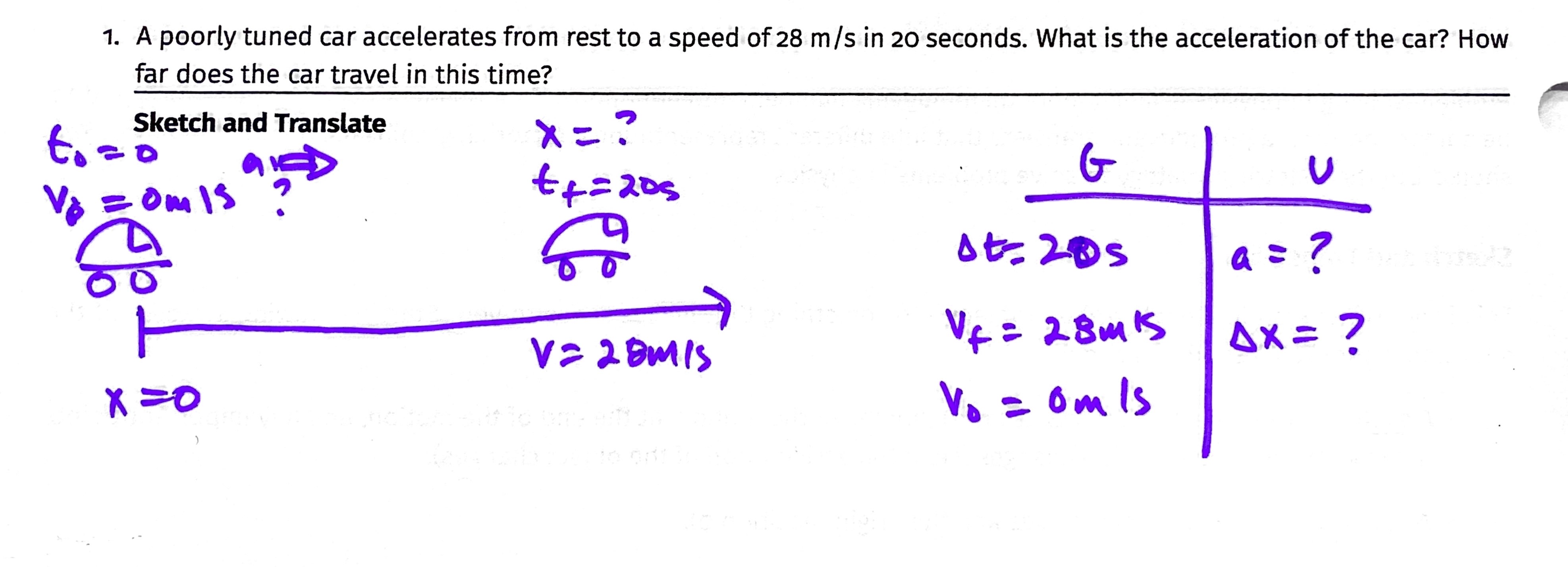
A poorly tuned car accelerates from rest to a speed of 28 m/s in 20 seconds. What is the acceleration of the car? How far does the car travel in this time?

🚨 Remember to:

  1. Sketch and Translate
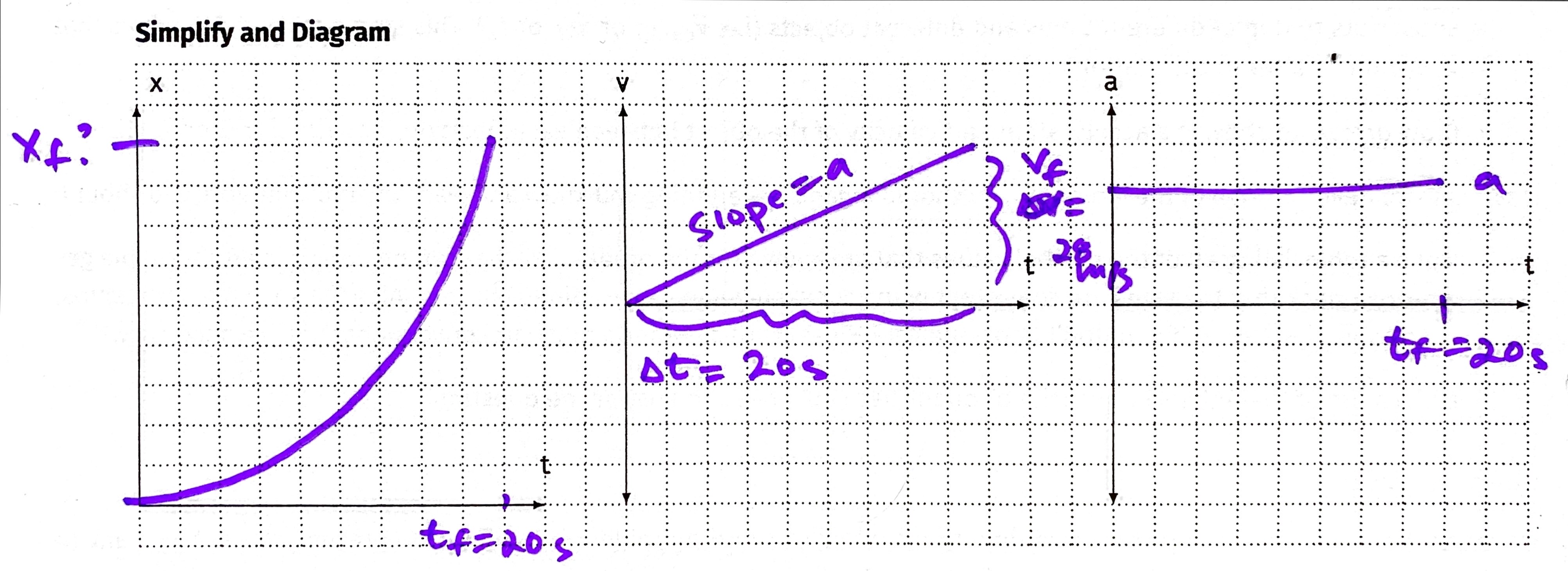
  2. Simplify and Diagram
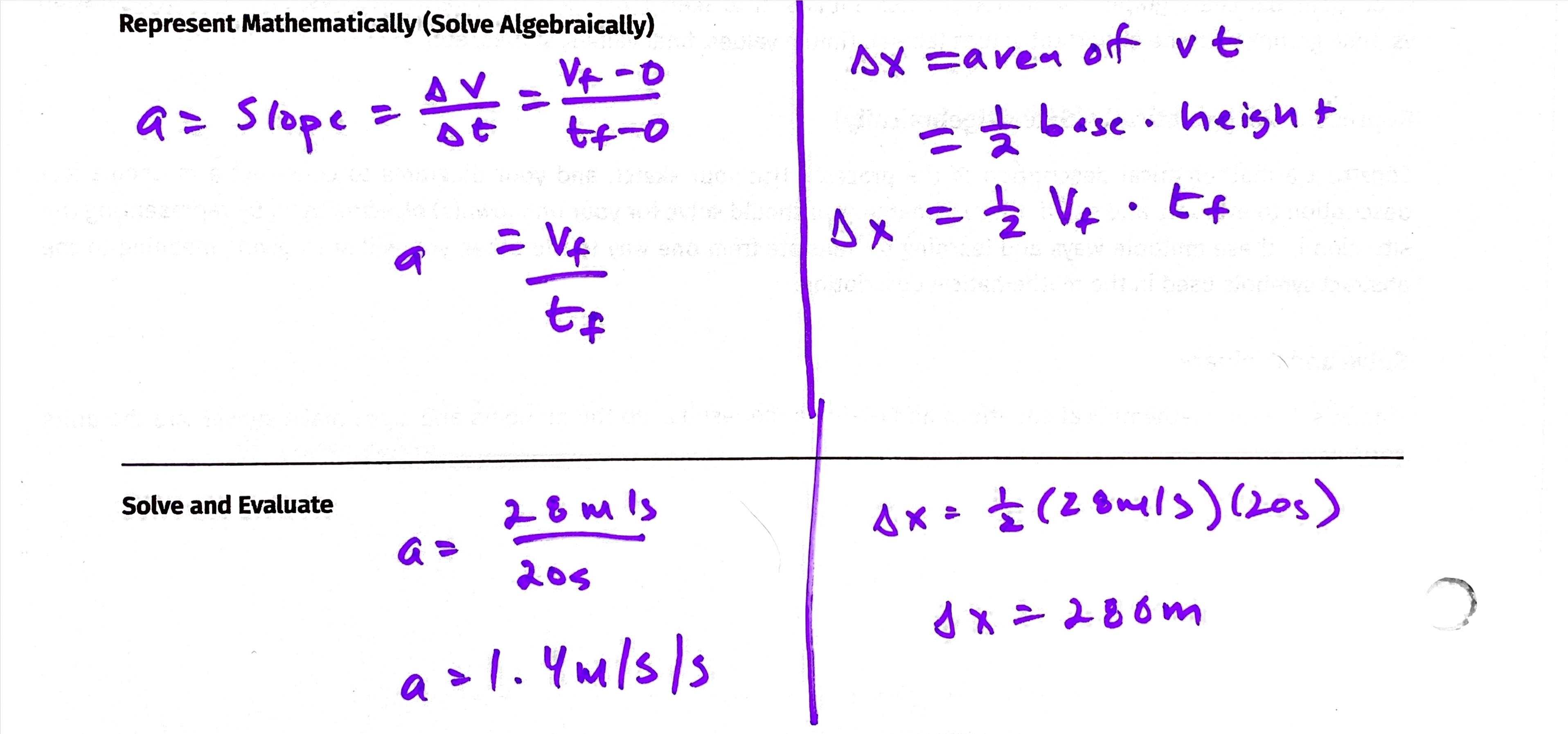
  3. Represent Mathematically
  4. Solve + Evaluate

🔎 Hint:

Use a graph or graphs to solve the problem.

Multiple Representations:

  • Verbal: Describes the motion of the car in a narrative manner.
  • Pictorial: A picture shows the initial and final motion of the car.
  • Diagrammatic: The picture is simplified and shows the motion of the car over multiple clock readings.
  • Graphical: Three representations that show how the position, velocity, and acceleration of the car vary over time.
  • Mathematical: Describes the velocity of the car as a function of time and the position of the car as a function of time.

Problem Solving Process:

  1. Sketch and Translate
  2. Simplify and Diagram
  3. Represent Mathematically
  4. Solve + Evaluate

1. Sketch

  • A sketch of the object or objects at the beginning of the motion, at the end of the motion, and any important points in between where the motion changes (i.e. if the acceleration of the object changes).
  • A coordinate system Label the axes and the origin (position 0).
  • Symbols that represent the time, position, and velocity of each object at each moment you have draw above. Use subscripts to depict different times and different objects (i.e. or or ). This step defines the symbols that you will use later in calculations.
  • Draw arrows to show the acceleration and velocity of the object between each position (or write or )

1. Translate

Now that you have a sketch of the situation you should organize everything you know and want to find. Therefore you should:

  • Make a table listing all of the symbol values that are known for the problem or that can be determine from simple geometry. Check that the signs are consistent with your sketch and its coordinate system. Also list known relationships, such as , even if you don't know the values yet. At this point do any unit conversions that are necessary.
  • Make a list of the unknown quantity or quantities you'll need to answer the question.

2. Simplify and Diagram (Physics Diagrams)

  • From our sketch we will no create physics diagrams...for motion this includes:
    • position vs. time graph
    • velocity vs. time graph (most useful)
    • acceleration vs. time graph

3. Represent Mathematically

  • mathematical description of the process
  • turn physics diagrams into equations:
    • use area of v-t to calc displacement
    • use slopes to calculate velos, or accelerations
    • use position functions to find final positions

4. Solve + Evaluate

  • substitute in given quantities and solve!
  • Evaluate: does this number make sense? Is it a reasonable solution?

Example:

A poorly tuned car accelerates from rest to a speed of 28 m/s in 20 seconds. What is the acceleration of the car? How far does the car travel in this time?

Sketch and Translate


Simplify and Diagram


The Kinematic Equations

This is the equation of the line for a velocity vs. time graph

  • = "final velocity" or velocity at time
  • = "initial velocity" or velicity at time = 0
  • = acceleration
  • = time

or

Function of a position vs. time graph

  • = "final position" or position at time
  • = initial position or position at time = 0
  • = "initial velocity" or velicity at time = 0
  • = acceleration
  • = time

  • = "final position" or position at time
  • = initial position or position at time = 0
    • Note: = displacement of object
  • = "final velocity" or velocity at postion
  • = "initial velocity" or velicity at
  • = acceleration

Kinematic Equations

...from AP Reference Table

  • the subscript indicates the plane of motion, these equations also work for and planes of motion
  • we will often remove that subscript when writing equations involving problems with only one plane of motion: i.e.

Kinematic Equations

Reminder:

so...

  • becomes ➡️
  • becomes ➡️

...one more...not on reference table

the area of a trapezoid for a V-T Graph:

  • useful if you don't know acceleration, but know initial, final velocity and time

Kinematic Cross Diagram for Problem Solving

center

Kinematic Cross Diagram

center

Identifying Equations

center

Non-reference Table Equations

center

Using the Cross Diagram

  1. Setup
    1. Write down the cross
    2. Write down the known variables and underline those variables in the cross
    3. Star (or circle) the variable that is unknown and is being solved for
  2. Planning
    1. Circle the variables that are involved in this problem
    2. Use the equation that involves those four variables
  3. Execution
    1. Solve the problem
    2. You can circle twice: solve for first unknown to use in second equation

Example

A poorly tuned car accelerates from rest to a speed of 28 m/s in 20 seconds. What is the acceleration of the car? How far does the car travel in this time?

Try It:

0. An airplane accelerates down a runway at 3.20 m/s2 for 32.8 s until is finally lifts off the ground. Determine the distance traveled before take-off.

1. Kent Belate is driving down I-294 at 32.0 m/s. He accelerates at a uniform rate of 5.06 m/s/s over a distance of 58.1 m. How much time is required to cover this distance? (Hint: two steps)

2. A military aircraft accelerates from rest for 4.03 seconds to take off of an aircraft carrier along a 82.6-m runway. Determine the take-off speed of the plane.

center


More Complicated Example

Gideon is South's best speed skater. He accelerates from 0.00 m/s to 7 m/s in 5 s and then continues at this constant speed for another 8 s. What is the total distance Gideon skates?

Practice

A speedboat increases its speed from 14.3 m/s to 31.1 m/s in a distance of 274 m. Determine the time over which this acceleration occurs.

center

1. 0-2, 4-6 2. 2-3 & 5-6 3. ~0.67 s 4. 6 m/s, 0, -3 m/s 5. Change after 3 seconds

Distance: 18 m Displacement: 6 m Avg. Speed: 3 m/s Avg. Velocity: 1 m/s North

═══════════════════════════════════════════════════════════════════ AREA UNDER A VELOCITY–TIME GRAPH — insertable slide block Unit 1, Kinematics. Pairs with area_under_vt_graph.pdf (13 Q, 11 pp). HOW IT RUNS: SLIDES 1–3 set the activity up, before the worksheet goes out SLIDES 4–6 how to draw the low / high / midpoint rectangles — show when the class reaches that part of Q5 SLIDES 7–25 the summary: what they did and what they found. One continuous run, AFTER the worksheet is finished. Slides 7 on are a recap, not a reveal. They are written to be read back to a class that has already done the work, in the order they did it. Figures are the vt_*.svg files in this folder. ═══════════════════════════════════════════════════════════════════

Deliberately NOT titled "area under the curve." The title is the question students are about to answer for themselves.

Warm-up, 2 minutes, everyone gets it. Do NOT point out that 24 is also the rectangle's area — the worksheet walks them into that in Q1(c)–(d).

Say the last line out loud, then hand out the worksheet. The next three slides are for the moment the class reaches the bracketing in Q5. Everything after those waits until the worksheet is done.

───────────────────────────────────────────────────────────────── HOW TO DRAW THE RECTANGLES — show when the class reaches the bracketing in Q5, to the whole room or one group at the board. This is technique, not the answer: the demo line is not the Q5 line, it starts above zero and its axes carry no numbers, so nothing here can be copied into the table. ─────────────────────────────────────────────────────────────────

This is the step the first group could not find on their own. They were trying to draw a rectangle before deciding what its height should be. Ask: "over this one slice, what is the slowest the cart ever goes?" Nothing here reveals the answer — the demo line is not the Q5 line.

The point to land: you are not choosing a good estimate, you are choosing a guaranteed-wrong one, twice, in known directions. That is what a bracket is.

Step 5 is worth saying twice: every rectangle in a round has the SAME width, so the sum is (sum of heights) x delta-t. Groups that miss this multiply each height separately and lose the thread in arithmetic. The falling-line note is for Q6, and for Object A in Part C.

THE SUMMARY STARTS HERE — run slides 7 to 25 straight through once the worksheet is done. If you collected group wordings from Q7, read one or two aloud here before moving on; the rest of the run answers them.

This is the slide worth slowing down on. Two follow-ups for the room: - Panels are laid out to match the worksheet: position on the left, velocity on the right, time axes aligned so you can read straight across. - Ask: is the x–t graph steepest where the v–t graph is lowest? (No — steepest where v is HIGHEST. Let them catch it themselves.) - Slope of each x–t segment = 8, 2, 5 m/s. The velocities, handed back.

Q3. This is where the sign rule was actually built, and it was built on RECTANGLES on purpose — no sloping line, no changing velocity, nothing else to think about at the same time. The question to re-ask here: "your question-2 rule said find the areas and add them up. Which of these three is a problem for that?" Then the payoff on the left: +12 and -12 cancel, so at t = 5 s the cart is back where it started, and BOTH graphs say so — the position graph touches zero, the velocity graph has equal areas on opposite sides. Displacement over the 8 s is +6 m; distance travelled is 30 m.

This is the step the sequence used to skip. Students had done the slicing without ever being told why slicing helps. The argument in one breath: the formula is fine, it just needs a constant v; so manufacture one, slice by slice, and choose it so you know which way you are wrong. Everything after this is bookkeeping.

Four slices — one row of the table they filled in. This comes BEFORE the squeeze on purpose: settle what the three methods are at a single slice count, then show what refining does to them. Ask before you advance: why is the third one exact? Because on each slice the rectangle pokes ABOVE the line on the left half by exactly as much as it falls BELOW on the right half — congruent triangles, which is only true because the graph is a straight line. The worksheet's "Midpoint" column averaged the two bounds; this slide uses the mid-slice velocity instead. For a straight line they agree, and both give 36.

What this slide is FOR: it is the payoff of the previous one. Each rectangle is still wrong, but the amount it is wrong by shrinks with the slice. Ask for the two observations before you say anything: (1) the gap halves (2) the midpoint never moves

The honest footnote to slide 13: the straight line was the easy case. Ask what is DIFFERENT here. The answer worth extracting: the midpoint is no longer exact. On a straight line the bit poking above the curve and the bit missing below were congruent triangles and cancelled perfectly. On a curve they only NEARLY cancel — 21.50, then 21.375, then 21.344, closing on 21.33 without ever landing on it. Good enough is not the same as exact. AP 1 does not ask for quantitative work on non-uniform acceleration, but the CED does expect students to analyse such situations qualitatively — this slide is that, and it is where the idea goes in calculus.

If a group's Q6 wording dropped "time axis" or dropped the sign, this is the moment to show why each phrase is there rather than asserting it.

The sloping-line version of *Backwards Counts Too*. They built the sign rule there, on rectangles; here it has to survive a triangle and a zero crossing. Ask what changed, and settle on "nothing: only how much region there is and which side of the axis it sits on."

This is the distinction that decays fastest — plan to re-ask it cold on the warm-up two days from now.

The hinge of the summary: everything from here is Part C, and the point is that none of it needed a new rule. Ask what they had to do differently. The honest answer is "nothing, except watch the sign."

Read it as a matrix, not four unrelated pictures: - ROW picks the sign of the acceleration, and that sets which way every curve in the row bends. - COLUMN picks slowing vs. speeding, which is about the SIGNS MATCHING, not about the sign of a on its own. The velocity graph on the right is the whole row at once — left of the dashed line it is slowing, right of it, speeding up. Same straight line.

# Sketch and Translate ![center](../figures/Sketch.jpg) --- # Simplify and Diagram ![center](../figures/Diagram.jpg) --- # Represent ➡️ Solve: ![center](../figures/Solve.jpg) ---
───────────────────────────────────────────────────────────────── REDRAWN versions of the three handwritten figures above — same worked example, same four steps, rebuilt in the style of the vt_*.svg figures from the area-under-a-VT-graph block. Here for comparison: keep one set and delete the other three. ─────────────────────────────────────────────────────────────────

Linger on the middle panel. That shaded triangle is the displacement, and it is the same area rule they built for themselves earlier — handed back to them inside a problem they are now solving.

Left column is slope (v-t graph), right column is area (v-t graph). Same graph, two different tools — the "Two Graphs, Two Tools" slide, cashed out on a real problem.

Don't explain it yet. Put it up, name the five, and ask what is missing from the list (nothing is — that is the point). The payoff lands on the next few slides when they see each equation is a loop around four of them.

The greyed-out variable is the one the equation cannot help you with. Ask it as a question: "which one is missing from this loop?" before you show the equation underneath.

The right-hand one is the odd shape: a ring that goes around 'a'. That is the trapezoid-area equation from the v-t graph — the one they built themselves back in the area block. Worth naming out loud.

Known: v0, vf, dx. Wanted: dt. That is four quantities, and the one left out is 'a' — so it is the ring equation, dx = 1/2(v0 + v)dt. Let them find that from the cross rather than telling them.